Quantpedia Composite Seasonality in MesoSim
Introduction
The Environment friendly Market Speculation (EMH), concept developed within the Nineteen Sixties, states that inventory costs replicate all accessible data, making it not possible to persistently earn above-average returns utilizing this data. Nonetheless, quite a few research problem this view by documenting anomalies that counsel markets will not be totally environment friendly. One group of such anomalies, often called calendar anomalies, exhibit predictable patterns in inventory returns linked to particular instances.
Motivation
In one among our older posts titled ‘Case Research: Quantpedia’s Composite Seasonal / Calendar Technique,'[11] we provide insights into seasonal buying and selling methods such because the Flip of the Month, FOMC Assembly Impact, and Possibility-Expiration Week Impact. These methods, freely accessible in our database, usually are not solely examined one after the other, however are additionally mixed and explored as a cohesive composite technique. In partnership with Deltaray, utilizing MesoSim — an choices technique simulator identified for its distinctive flexibility and efficiency[5] — we determined to discover and quantify how our Seasonal Technique performs when utilized to choices buying and selling. Our motivation is to analyze whether or not this technique might be improved by way of danger and return. We purpose to systematically harvest the VRP (volatility danger premium) timing the entries utilizing calendar technique to keep away from traditionally detrimental buying and selling days.
Within the following sections, we’ll briefly talk about tutorial research within the space of calendar anomalies, we then describe the information preparation course of and the 4 steps concerned in creating our remaining technique.
Relationship to Literature
As early as 1962, Osborne noticed an fascinating weekly sample: U.S. inventory markets expertise considerably decrease returns on Mondays and better returns on Fridays in comparison with different weekdays[6]. Traders have been eager on exploiting related temporal anomalies ever since. Constructing on this, the January Impact, documented by Rozeff and Kinney in 1976, reveals that returns in January are unusually excessive in comparison with different months[7]. Additional increasing on month-to-month developments, Ariel highlighted the Flip-of-the-Month Impact, the place the tip of 1 month and the beginning of the following usually see greater returns, suggesting an optimum technique of shopping for SPY ETFs at month’s finish and promoting originally of the following[2]. The Payday Impact, much like the Flip of the Month, is triggered round typical payday schedules, significantly on the fifteenth and at month-end, when staff typically make investments their paychecks[4]. This affords one other worthwhile alternative to purchase SPY ETFs on nowadays and promote them shortly after. Moreover, the market displays predictable patterns round particular occasions akin to Federal Open Market Committee (FOMC) conferences, the place the S&P 500 usually performs higher, presumably in response to the Federal Reserve’s choices geared toward stabilizing and enhancing the financial system[9]. By buying SPY ETFs the day earlier than an FOMC assembly and promoting them afterward, traders can capitalize in the marketplace’s usually optimistic response. One other buying and selling window is the Possibility-Expiration Week Impact, noticed throughout the week main as much as the common expiration of choices—the Friday earlier than the third Saturday of every month. Throughout this era, shares with giant market capitalizations and energetic choices buying and selling are inclined to yield greater returns[8].
These patterns are only a few examples of the numerous calendar results noticed globally, which vary from these associated to the Islamic calendar[1] to occasions just like the FIFA World Cup[3]. Every highlights potential inefficiencies in market habits. Such results considerably form our fashionable buying and selling methods. Via our collaboration with Deltaray, we discover these anomalies to develop methods that would result in higher risk-adjusted returns with concentrate on choices buying and selling.
Knowledge Preparation
First, we created a Google Sheet for our information, the place every row represents a date.
Column A contains dates throughout the backtest time vary, every marked with a 9:30 AM timestamp. This timing ensures that MesoSim can use the information on the identical day.
Column B tracks when common choices expire. We use a components that checks if the date in Column A is the third Friday of the month. Third Friday of the month is when these choices usually expire. If there’s a match, the date is marked with a ‘1’. Formulation runs as follows:
=if(date(Yr(A2), month(A2), day(A2)) = (DATE(YEAR(A2),MONTH(A2),1+7*3)-WEEKDAY(DATE(YEAR(A2),MONTH(A2),8-6))), 1, 0)
This components calculates if the given date aligns with the third Friday by subtracting the weekday variety of the second day of the month from the twenty second.
Column C, the ‘choice expiration week’, calculates and marks the entire week main as much as every expiration date utilizing the components:
=if(countif(B2:B6, “=1”) > 0, 1, 0)
If there’s a cell in a given vary that accommodates ‘1’, it signifies that the week contains an choice expiration day. Any week containing an expiration date is marked with a ‘1’.
Column D, the ‘choice expiration week begin’, indicators when the expiration week begins. This occurs when the marks in Column C change from ‘0’ (no expiration week) to ‘1’ (begin of expiration week) between two rows. This column will probably be utilized by MesoSim to set off trades Formulation:
=if(and(C2 <> C1, C2 = 1), 1, 0)
To see when one month adjustments to the following, we create a Column E ‘finish of the month’ utilizing the components:
=if(month(A2) <> month(A3), 1, 0)
This checks if the month of the present row is totally different from the following and marks the transition with a ‘1’.
On condition that the end-of-month interval is already lined by the Flip of the month represented by Column E, we additionally marked the mid-month payday, occurring across the fifteenth in Column G:
=if(day(A2) = 15, 1, 0)
Column F contains the dates of the FOMC (Federal Open Market Committee) conferences. These dates might be sourced from monetary calendars like Investing.com[10].
Our totally ready Sheet might be accessed right here: https://docs.google.com/spreadsheets/d/1hUo-De3z2QqLV5iL-X90a60sO0vXlCAY626ETTsZUOU/edit?usp=sharing
Method
The evaluation consists of 4 steps: organising artificial lengthy positions utilizing choices, making use of a volatility danger premium (VRP) technique, incorporating stop-loss mechanisms to handle dangers, and optimizing place sizing for higher danger administration. Every step will probably be described intimately.
Step 1: Artificial Lengthy utilizing Choices
In our authentic paper and backtest we use SPY ETF. As MesoSim is an option-only backtester, they use an artificial lengthy place on SPX to match the SPY-based funding technique. Artificial Lengthy consists of concurrently Shopping for a Name Possibility ATM and Promoting a Put Possibility ATM. These two actions mimic shopping for the SPY ETF and characterize a easy solution to replicate our technique utilizing choices.
Backtest outcomes might be seen right here: https://mesosim.deltaray.io/backtests/769b2a40-03b4-4ef3-b397-353f50ee0c01
QuantPedia Composite SyntheticLong Overview
Expiration choice
We use choices expiring nearest to five DTE in case of option_expiration_week_start and end_of_month indicators. For every other sign (fomc, payday) we decide 1 DTE choices.
Respective configuration part:
“Expirations”: [ { “Name”: “exp1”, “DTE”: “(option_expiration_week_start == 1 or end_of_month == 1) and 5 or 1”, “Min”: “1”, “Max”: “5”, } ]
Construction / Leg definitions
We use the Assertion Selector to choose strikes utilizing the underlying worth as goal for the short_put leg. The long_call leg will use the identical strike because the brief put leg, utilizing the leg_short_put_strike variable.
Respective configuration part:
“Legs”: [ { “Name”: “short_put”, “Qty”: “-1”, “ExpirationName”: “exp1”, “StrikeSelector”: { “Statement”: “underlying_price” }, “OptionType”: “Put” }, { “Name”: “long_call”, “Qty”: “1”, “ExpirationName”: “exp1”, “StrikeSelector”: { “Statement”: “leg_short_put_strike” }, “OptionType”: “Call” }
Entry definition
We will enter whenever the signals defined in the Google Sheet is set to 1. We use the column-names defined in sheets as variables:
fomc_today, end_of_month, option_expiration_week_start, payday
We allow one Position in flight and we try to enter every day, 5 minutes after open:
“Entry”: { “Schedule”: { “AfterMarketOpenMinutes”: “5”, “BeforeMarketCloseMinutes”: null, “Every”: “day” }, “Conditions”: [ “fomc_today == 1”, “end_of_month == 1”, “option_expiration_week_start == 1”, “payday == 1” ], “VarDefines”: {}, “AbortConditions”: [], “ReentryDays”: “1”, “Concurrency”: { “MaxPositionsInFlight”: “1”, “EntryShiftDays”: “1” }, “QtyMultiplier”: null },
Exit definition
We exit the commerce on the final buying and selling day. Alternatively, we might run it into settlement.
“Exit”: { “Schedule”: { “AfterMarketOpenMinutes”: null, “BeforeMarketCloseMinutes”: “5”, “Each”: “day” }, “MaxDaysInTrade”: “expiration_exp1_dte”, “ProfitTarget”: null, “StopLoss”: null, “Circumstances”: [], “VarDefines”: {} }
Exterior Knowledge and Simulator settings
We leverage MesoSim’s Exterior Knowledge capabilities to load the information ready in Google Sheet and use it as sign for entry. To have a practical simulation we set the Fee to $1.5 / contract and set the fill mannequin to Mid Worth. Slippage is disabled for this experiment:
“ExternalData”: { “CsvUrl”: “https://docs.google.com/spreadsheets/d/e/2PACX-1vRei87mgnKNW-1dehmQwYzipn47J8cyhPRsZom50J_jH5OY1jY23aOeD9sglzLph9sRUgf8qVbWAm3f/pub?output=csv” }, “SimSettings”: { “FillModel”: “AtMidPrice”, “SlippageAmt”: “0”, “Fee”: { “CommissionModel”: “FixedFee”, “OptionFee”: “1.5”, “DeribitCommissionSettings”: null }, “LegSelectionConstraint”: “None”, “Margin”: { “Mannequin”: “None”, “HouseMultiplier”: null, “RegTMode”: “CBOEPermissive” } }
As for outcomes, when evaluating the run with S&P Purchase and maintain efficiency we discover that the time in commerce is decreased to 1/third and Sharpe is elevated from 0.78 to 1.04.
Let’s transfer to the following step.
Step 2: VRP – Quick Put
To harness Volatility Danger Premium (VRP) we shifted from a Artificial Lengthy place to Quick Put. Quick Put is a bullish choices technique the place the premium might be collected if the underlying worth stays above the contract’s strike worth. As we talk about in our weblog put up about Volatility Danger Premium, the core of VRP is that implied volatility from inventory choices usually exceeds precise historic volatility. This means the potential to earn a scientific danger premium by short-term promoting of choices.
Leg definition
The brief put contract is chosen utilizing Delta-based strike selector. To keep away from promoting tail danger we goal contracts with Delta=10. Basically, Delta signifies how a lot the value of an choice is anticipated to maneuver per a one-point motion within the underlying asset.
“Legs”: [ { “Name”: “short_put”, “Qty”: “-1”, “ExpirationName”: “exp1”, “StrikeSelector”: { “Delta”: “10” }, “OptionType”: “Put” } ] }
The chance graph (left aspect graph beneath) reveals the chance profile of the place we took. The expiration strains within the danger graph reveals how the trades will develop over time utilizing the Black-Scholes-Merton mannequin.
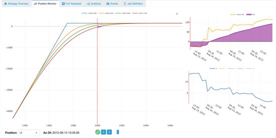
QuantPedia Composite ShortPut RiskGraph
Backtest run is on the market right here: https://mesosim.deltaray.io/backtests/229fe2c8-483c-4ab4-b8e4-403df2b7e6ed
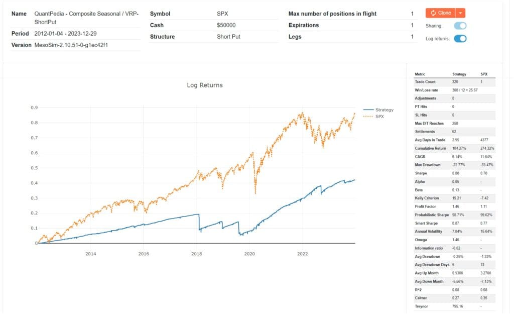
QuantPedia Composite ShortPut Overview
The outcomes present that volatility danger premium harvesting mixed with market timing is usually a extremely worthwhile majority of the time, however the rare losses can wipe multiplied days of earnings. The losses skilled throughout the above run had been linked to important market downturns, together with the dramatic inventory market occasions of 2018: Volmageddon and the worst U.S. inventory decline since 2008, in addition to the 2019 downturn pushed by the US-China commerce warfare.
Within the subsequent step, we’ll handle the rare losses utilizing an options-specific stop-loss mechanism.
Step 3: VRP – Quick Put with StopLoss
Controlling for danger is important in all buying and selling methods. There are a number of strategies to reduce draw back danger in options-based methods. You may resolve to exit or modify a place based mostly on:
Possibility moneyness, for instance, when the underlying worth falls beneath the strike worth.
Place Delta, for instance, if the delta exceeds 50.
The comparability of Revenue and Loss in opposition to the Credit score Obtained.
Different elements embody implied volatility (IV), different Greeks like theta, and market volatility indices akin to VIX or VVIX.
We are going to concentrate on exploring the primary three strategies intimately.
Possibility moneyness based mostly
When the underlying worth drops beneath the choice’s strike worth, e.g. when the Quick Put contract turns into In The Cash (ITM) the rate-of-loss of the place accelerates. It’s due to this fact logical to exit a place on the level (or earlier than) when the strike is breached. In MesoSim this may be outlined as:“Exit”: { “Circumstances”: [ “underlying_price < leg_short_put_strike” ], … }
Backtest run might be seen right here:https://mesosim.deltaray.io/backtests/26eb380b-abb4-48d1-91bd-2f16d3282c53
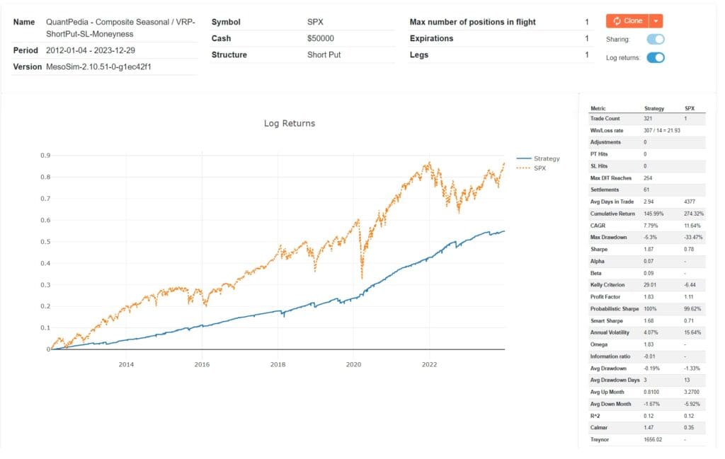
QuantPedia Composite ShortPut SL Moneyness overview
Delta based mostly
Delta values round 50 usually point out that an choices is someplace round At The Cash (ATM). Nonetheless, it’s essential to notice that an choice could not all the time precisely match a delta of fifty when it’s ATM because of various market circumstances and particular traits of the choice. Because the delta exceeds 50, the choice strikes additional into-the-money (ITM). To handle danger successfully and to exit a place when it’s delta turns into bigger than 50, you need to use the next Exit Situation in MesoSim:
“Exit”: { “Circumstances”: [ “pos_delta > 50” ], }
For additional insights, please discuss with our backtest run, accessible: https://mesosim.deltaray.io/backtests/38cc3635-cb09-4cca-b3ee-89a247ed0305
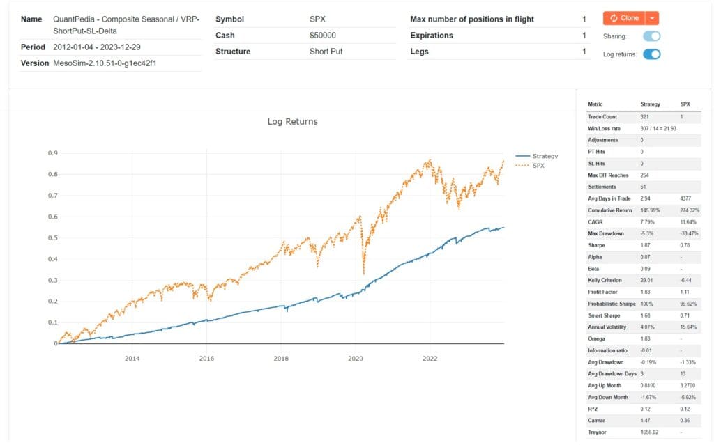
QuantPedia Compose ShortPut SL Delta overview
Observe that the curve is matching the Moneyness based mostly run because the Delta choice is matching the deltas of ATM choices.
Credit score acquired based mostly
Briefly-dated choice promoting methods the StopLoss is usually described as a perform of credit score acquired. You may resolve to exit a place if losses exceed a predetermined a number of of the preliminary credit score. To have a 2:1 Danger/Reward ratio we will set off a promote through the use of the Possibility Premium for the put we offered.
First we have to seize the Possibility Worth on entry:“Entry”: { “VarDefines”: { … “credit_received”: “leg_short_put_price * abs(leg_short_put_qty) * 100” }, … }
Then, we use the credit_received variable to exit when the place PnL reaches 2 instances of the worth: “Exit”: { “Circumstances”: [ “pos_pnl < (-1 * 2 * credit_received)” ], …}
For detailed efficiency metrics, please discuss with our backtest run: https://mesosim.deltaray.io/backtests/c395cb1a-7010-47b4-ae62-4796fbd51619
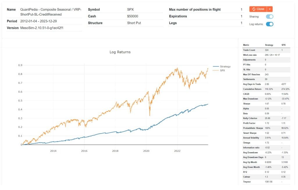
QuantPedia Composite ShortPut SL CreditReceived overview
The ultimate step includes making use of place sizing.
Step 4: VRP Sizing
The above runs used a set, preliminary account dimension of $50,000 for the commerce. That account dimension was chosen in order that the positions might be entered utilizing a Reg-T account. Choices are sometimes traded utilizing Portfolio Margin or SPAN based mostly margin accounts, which permit for larger leverage. On the time of writing, a ten delta Quick Placed on SPX requires $12,000 of shopping for energy for 1 Day to Expiration (DTE) and $9,000 for five DTE. Adopting a conservative technique, we use solely 50% of our purchasing energy, cutting down the preliminary money to $25k for the StopLoss based mostly trades.
The efficacy of this method is clear in comparison in opposition to the SPX, the place it achieves a comparable efficiency, however with decrease drawdown of 8.26% (versus 33.47%) and a extra favorable Sharpe ratio of 1.98 (in comparison with 0.77). Importantly, this technique is energetic available in the market solely 40% of the time, demonstrating its effectivity by limiting market publicity whereas nonetheless capturing important returns.
For detailed efficiency metrics and additional insights, please discuss with our current backtest run, accessible: https://mesosim.deltaray.io/backtests/460a6563-e35d-4296-9a83-a8f200737c84
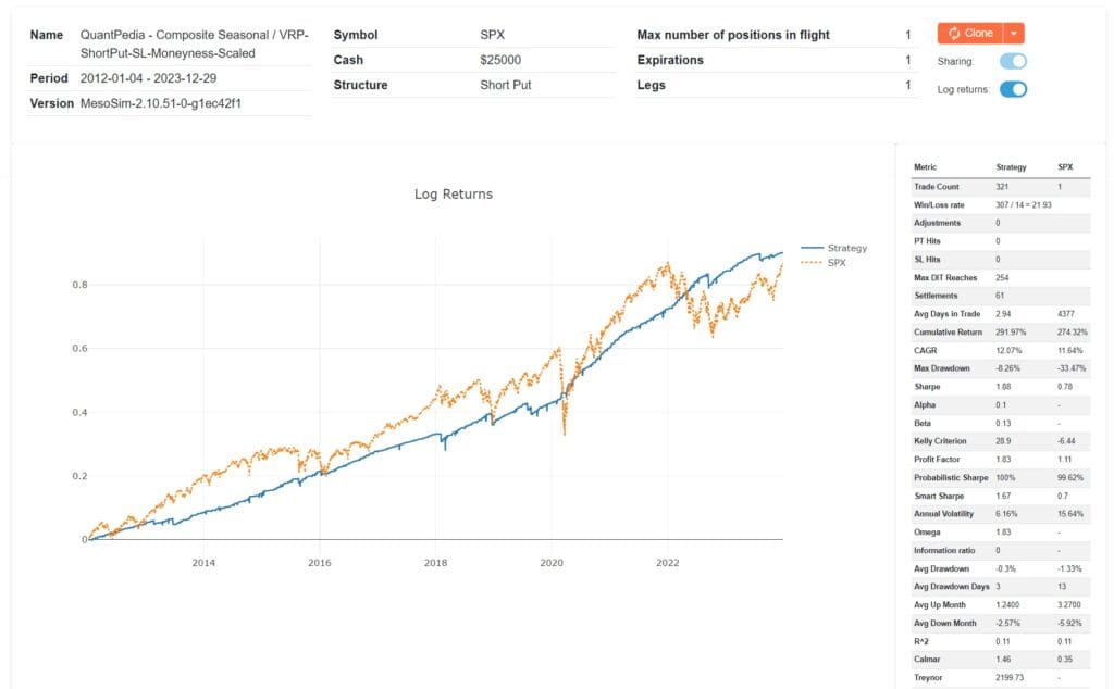
QuantPedia Composite ShortPut SL Moneyness Scaled
Conclusion
In collaboration with Deltaray, we utilized Quantpedia’s Composite Seasonal/Calendar Technique to choices buying and selling, gaining useful insights into how seasonal anomalies can be utilized within the choices market. Our principal purpose was to not solely replicate QuantPedia’s findings but in addition to reinforce them by successfully utilizing the Volatility Danger Premium (VRP).
Initially, we ready our information by marking essential market indicators akin to choice expirations and FOMC assembly dates. We then used MesoSim to simulate inventory holdings via artificial lengthy positions. After establishing a strong baseline, we examined the benefits of VRP with a Quick Put technique, discovering that though it typically results in important earnings, it additionally comes with the chance of extreme losses. To mitigate these dangers, we utilized StopLoss mechanisms based mostly on delta values, choice moneyness, and credit score acquired, which considerably improved our danger administration.
Our remaining method concerned utilizing the Quick Put technique and a conservative place sizing to optimize buying and selling circumstances. This improved our Sharpe ratio and Drawdown metric when in comparison with SPX.
Future work will refine our methods additional via sensitivity analyses and by including hedging part, particularly lengthy places.
Deltaray’s MesoSim is an choices technique simulator with distinctive flexibility and efficiency. You may create, backtest, and optimize choices and buying and selling methods on fairness indexes and crypto choices at a lightning-fast pace. Now, it’s built-in with ChatGPT to help customers in creating backtest job definitions.
Solely, just for the Quantpedia group, our readers can now use the coupon code QUANTJUNE to acquire a 30% low cost on new annual subscriptions for each the Customary and Superior Plans. The coupon is legitimate between thirteenth June and twentieth June 2024.
Are you on the lookout for extra methods to examine? Join our publication or go to our Weblog or Screener.
Do you wish to study extra about Quantpedia Premium service? Examine how Quantpedia works, our mission and Premium pricing supply.
Do you wish to study extra about Quantpedia Professional service? Examine its description, watch movies, evaluate reporting capabilities and go to our pricing supply.
Are you on the lookout for historic information or backtesting platforms? Examine our checklist of Algo Buying and selling Reductions.
Do you might have an thought for systematic/quantitative buying and selling or funding technique? Then be a part of Quantpedia Awards 2024!
Or observe us on:
Fb Group, Fb Web page, Twitter, Linkedin, Medium or Youtube
References
[1] ALMUDHAF, Fahad. The Islamic calendar results: Proof from twelve inventory markets. Accessible at SSRN 2131202, 2012.
[2] ARIEL, Robert A. A month-to-month impact in inventory returns. Journal of monetary economics, 1987, 18.1: 161-174.
[3] EHRMANN, Michael; JANSEN, David-Jan. The pitch moderately than the pit: investor inattention throughout FIFA World Cup matches. 2012.
[4] Ma, Aixin and Pratt, William Robert, Payday Anomaly (September 28, 2018). Accessible at SSRN: https://ssrn.com/summary=3257064 or http://dx.doi.org/10.2139/ssrn.3257064
[5] MesoSim portal by Deltaray. MesoSim Portal by deltaray. (n.d.). Accessible at: https://mesosim.deltaray.io/
[6] OSBORNE, Maury FM. Periodic construction within the Brownian movement of inventory costs. Operations Analysis, 1962, 10.3: 345-379.
[7] ROZEFF, Michael S.; KINNEY JR, William R. Capital market seasonality: The case of inventory returns. Journal of monetary economics, 1976, 3.4: 379-402.
[8] Stivers, C., & Solar, L. (2013). Returns and choice exercise over the option-expiration week for S&P 100 shares. Journal of Banking & Finance, 37(11), 4226-4240.
[9] Tori, C. R. (2001). Federal Open Market Committee conferences and inventory market efficiency. Monetary Providers Evaluate, 10(1-4), 163-171.
[10] U.S. Federal Reserve (FED) assembly minutes. (n.d.). Investing.com. Accessible at: https://www.investing.com/economic-calendar/fomc-meeting-minutes-108
[11] Vojtko, R., & Padyšák, M. (2019, April 26). Case research: Quantpedia’s composite seasonal / calendar technique. QuantPedia. Accessible at: https://quantpedia.com/quantpedias-composite-seasonalcalendar-strategy-case-study/
Share onLinkedInTwitterFacebookConsult with a pal


